Simulate an experiment

This section describes how to simulate experiments without access to the scanner. This is very useful during software development and testing, as all functionalities can be tested without having to request scanner time.

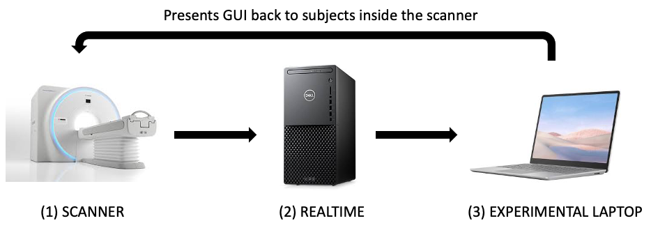
During an experiment, there are three different computers involved. Data flows in the following manner.

First, the scanner (1) acquires images and sends them to the realtime system (2).

For each incoming EPI image, the realtime system performs the following operations:

alignment towards reference volume
estimation of head motion
extraction of data within a mask.

Both motion parameters and extracted voxel-wise values within the mask are subsequently sent via TCP/IP to the experimental laptop (3).

The experimental laptop takes incoming data, does additional pre-processing, and then drives the experiment GUI based on how that incoming data looks like a series of pre-defined templates.

When developing this software, we will need to simulate the workings of these three systems, but using a single machine (our development machine). The rest of this section describes how to accomplish this process.

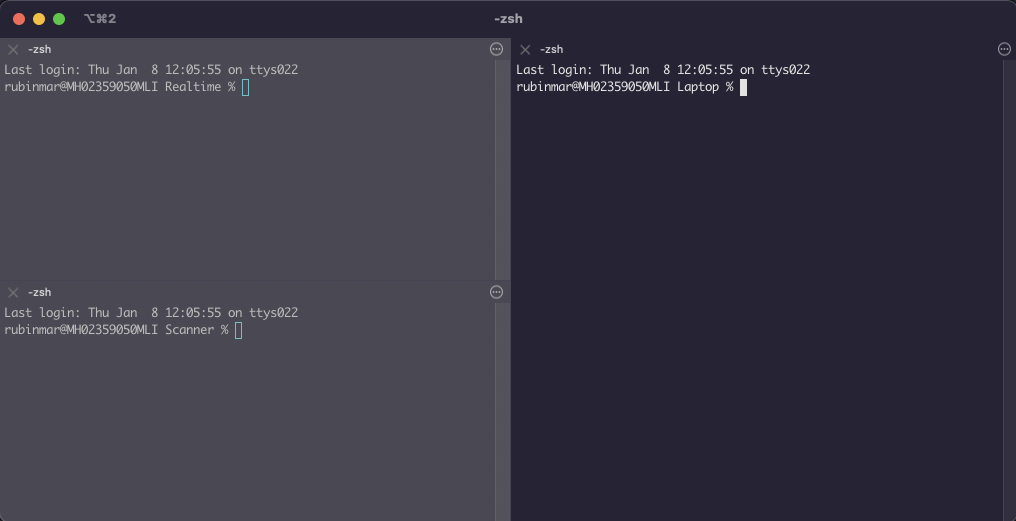
1. Open three different Terminals on your laptop in the Simulation/ directory, then cd to the following directories:

Scanner: you will use this window to simulate the scanner sending data to AFNI realtime
Realtime: here you will start AFNI in realtime mode. It will take incoming data from the “fake” scanner, and after a few things sending on its way to the rtcog software.
Laptop: here you will start the rtcog software.

Download the sample data

Enter the empty Scanner folder.
Download sample datasets to the Scanner folder.

To a minimum you should have an anatomical dataset, a short EPI dataset to use as reference for alignment, and then two additional long EPI datasets: one will be used for training the classifier and the second one to simulate a real experience sampling run.

Go to the Realtime teminal:

Enter the empty Realtime folder.
Copy the 01_BringROIsToSubjectSpace.sh script here.
Copy the Frontiers2013_CAPs.nii file here.
Export the following variables

export AFNI_REALTIME_Registration=3D:_realtime
export AFNI_REALTIME_Base_Image=2
export AFNI_REALTIME_Graph=Realtime
export AFNI_REALTIME_MP_HOST_PORT=localhost:53214
export AFNI_REALTIME_SEND_VER=YES
export AFNI_REALTIME_SHOW_TIMES=YES
export AFNI_REALTIME_Mask_Vals=ROI_means
export AFNI_REALTIME_Function=FIM

Start AFNI in realtime mode

$ afni -rt

Simulate acquisition of anatomical dataset

On the Scanner console, type:

rtfeedme Anat+orig

By the end of this step, you should have a new dataset (rt.__001+orig) that contains the anatomical data (but now in the realtime system) in the Realtime folder.

Simulate acquisition of the EPI reference dataset

On the Scanner console, type:

rtfeedme EPI_Reference+orig

By the end of this step, you should have a second dataset on Realime (rt.__002+orig) on the Realtime folder that contains the EPI reference data (but now in the realtime system)

Pre-process Anatomical and bring masks to EPI Reference space

Go to the Realtime terminal
Run 01_BringROIsToSubjectSpace.sh as follows:

sh ./01_BringROIsToSubjectSpace.sh \
       rt.__002+orig. \
       rt.__001+orig. \
       Frontier2013_CAPs.nii

This will generate a lot of new files. The key ones moving forward are:

EPIREF+orig: this will become our reference volume for realtime alignemnt.
GMribbon_R4Feed.nii: this will be our mask for sending data to the laptop.
Frontiers2013_R4Feed.nii: this will be our CAPs template aligned to the EPI data.

The last two files need to be transfered (i.e., copied) to the Laptop directory.

$cp ${REALTIME_FOLDER}/GMribbon_R4Feed.nii ${LAPTOP_FOLDER}
$cp ${REALTIME_FOLDER}/Frontiers2013_R4Feed.nii ${LAPTOP_FOLDER}

Configure the realtime plugin for the rest of the experiment.

In the main AFNI window, click on Define Datamode –> Plugins –> RT Options

On the new window, ensure the following configurations:

Registration = 3D: realtime
Resampling = Quintic
Reg Base = External Dataset
External Dset = EPIREF+orig
Base Image = 0
NR = 1200 (Or as many volumes as you are expecting in the next run)
Mask = GMribbon_R4Feed.nii
Val to Send = All Data (light)

Start rtcog in Basic mode in the Laptop terminal.

See Usage for instructions.

Simulate acquisition of the training run

In the Scanner console, type:

rtfeedme TrainingRun+orig

The data will be send to AFNI, who in turn will do motion correction (towards the EPI reference dataset), and then send the values of each voxel in the GMribbon mask to the rtcog program that is listening by default on port 53214. By the end of this step, in the Laptop folder you should have the following files:

$prefix_Options.yaml: record of all the options.
$prefix.Motion.1D: motion estimates.
$prefix.Zscore.nii: final per-TR activity map?
$prefix.pp_EMA.nii: data following the EMA step.
$prefix.pp_iGLM.nii: data following the incremental GLM step.
$prefix.pp_iGLM_$regressor.nii: fitting (beta value) of each nuisance regressor.
$prefix.pp_LPfilter.nii: data following the low pass filtering step.
$prefix.pp_Smotth.nii: data following the spatial smoothing step.

Train the SVR

Select the templates of interest and create a txt file with labels. The txt file should be comma-separated and in the same order as your templates file. For example:

3dTcat -prefix Templates_R4Feed.nii Frontier2013_CAPs_R4Feed.nii"[25, 4, 18, 28, 24, 11, 21]"
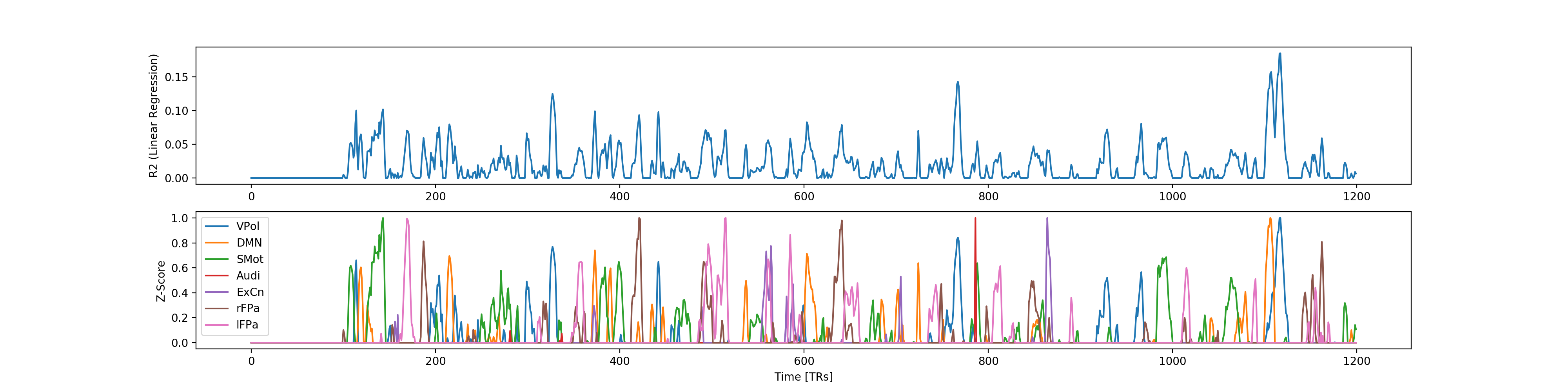
echo "VPol,DMN,SMot,Audi,ExCn,rFPa,lFPa" >> template_labels.txt

Go to the Laptop terminal and run:

python rtcog/matching/offline/svr.py \
      --data path/to/training_data.nii \                   # The final preprocessed data from Basic run
      --mask path/to/your_mask.nii \                       # Your mask file
      --templates_path path/to/your_templates.nii \        # The templates of interest
      --template_labels_path path/to/template_labels.txt \ # The names of your templates
      --out_dir ./output_directory  \                      # Where results will be saved
      --prefix training_svr \                              # Prefix for output files
      --no_lasso

This will generate the following additional files in the Laptop folder:

training_svr.pkl: trained SVRs (needed for the rest of the experimental runs)
training_svr_training_vols.csv: ?
training_svr_lm_R2.csv: R2 for linear regerssion on training data
training_svr_lm_z_labels.csv: TR-by-TR labels of SVRs (after Z-scoring)
training_svr.png: static summary of SVR traning
training_svr.html: dynamic summary of SVR traning

Here is an example of the static training report

Instead of training SVRs, you can also use the mask method for spatial matching.

python rtcog/matching/offline/mask.py \
       --data path/to/training_data.nii \                   # The final preprocessed data from Basic run
       --mask path/to/your_mask.nii \                       # Your mask file
       --templates_path path/to/your_templates.nii \        # The templates of interest
       --template_labels_path path/to/template_labels.txt \ # The names of your templates
       --out_dir ./output_directory  \                      # Where results will be saved
       --prefix mask_method \                               # Prefix for output files
       --template_type binary \                             # Template type: "binary" or "normal"
       --thr 10 \                                           # Threshold (float) to use for the templates

This will generate the following additional files in the Laptop folder:

mask_method.template_data.npz: template data (needed for the rest of the experimental runs, to be passed in with --match_path argument)
mask_method.act_traces.npz: The activity traces from this method
mask_method.traces.png: static summary of the activity traces
mask_method.traces.html: dynamic summary of the activity traces

Using the output of this method, decide on a threshold to use in the experimental run (--hit_thr)

Run rtcog in ESAM mode

Now that you have trained the SVR (or created the mask method templates), you can simulate a real experience sampling run. First set match_method in the config yaml to either svr or mask_method depending on which approach you are using.

Then, start the experiment. Refer to Usage for instructions. Note that the input for --match_path will be:

training_svr.pkl for SVR method
mask_method.template_data.npz for mask method

NOTE: This doc is a work in process